Explanation

This model will introduce you to basic elements of the Planimate® platform and also provide some initial experience with some important general concepts concerning the dynamic behaviour of systems.

We are going to take a look at a simple system and its dynamics.

The major dynamic events of this system will be as follows:

Arrivals	= Entry into System.
Waiting Around	= Queuing for Service.
Processing	= by a Server.
Departure	= Exit from System.

The thing to appreciate here is:

• We want to make a model of a system to see, learn or show others how it works.
• In this system, events occur and it changes over time.
• Hence the model must be dynamic.

Imagine we could isolate an area in a real system (e.g. a set of office cubicles), then watch and record what happens in it.

A video recording is one possible strategy for recording a system’s activities. To fully cover the system area, you may need many simultaneous recording streams. And what would you record - the people or the paper?

You would then also need to set up an array of screens for the viewer to watch the playbacks.Too many screens and not enough eyes makes forming a useful understanding of cause and effect in this system very elusive. And even then, there is still a need to be able to communicate this behaviour to others, so that they can understand it, before you can then fruitfully discuss future options for the system.

To be able to give this information to somebody else to review, some kind of language is needed to represent how the events going on in that system relate to each other, things like:

• what causes what,
• what waits for what else,
• what becomes what else,
• what decisions are made,

… and much more.

With a standard language for this, we can use a machine (the PC) to build this system model.

This is highly useful, because in this kind of machine we can use the language to reconfigure our system model to represent a variety of current interpretations of, or future options for the system being examined. These representations can be stored, transmitted, and reproduced in other machines, in other locations, before other eyes.

Planimate® is a language for specifying the elements and behaviours of a dynamic system.

Hands On

Launch Planimate and explore it a little.

Maximize the window.

Load a simple model from the Intro Folder

Press a few buttons, run it etc, look around…

Start a New Model (Discard current)

If not already visible, show the Object Palette / sidebar (View / Object Palette).

You can drag objects off the palette or click them and then click where you want them.

Drag them about,

Rename them by clicking on the names.

Right-click on them to produce their editing menu.

Delete them.

Copy and Paste them.

Save, and then start a New model.

Now for your first Planimate® model - a Distribution Centre.

Change to Object View <Ctrl+O>.

Make the Clock visible using View / Simulation Clock.

Your mouse pointer should look like:

From the object palette, Add an:

Entry	Items cross the system boundary and enter a system from an Entry. (NB: an Entry has no Capacity)
Queue	Items wait in Queues to access other objects.
Multiserver	We use the default Single Capacity (only holds one thing). Rename it to “Load or Unload”.
Exit.	Items leave the system through the exit, it is another boundary. (NB: an Exit has no Capacity)

Line them up from left to right. These are the objects of our system.

Save your Model (We will call this Model DC01).

Reflect on the question: “Where is the DC?”. Next we need to define the items that will move through and interact with these objects in the DC.

Go to Menu Bar / Edit / Item Classes / Add New Item Class.

Give it the name “Vehicle”

Notice the following things:

• An Item icon appears in the Item Palette.
• The mouse pointer changes to show:
• (Flow) indicator in Planimate®’s Window Title.

Now create a path from Entry > Queue > Server > Exit by clicking on each in turn, from left to right.

Type Ctrl-O to get back to object mode and save the model.

Run the Model. One item will move across the model. OK the dialog that announces the model has finished.

To make things more interesting, right click the Entry and select Mode. Select “Periodic Arrivals” from the list. OK and run the model again.

Observations

Now it is time to study the model and make and discuss observations, so you get a better understanding of the language being used in a Planimate® dynamic model.

Here are some questions for you to examine:

• Can you explain what the clock is doing?
• Can you identify the different “Events” in this simulation?
• Does the clock “Tick” during Animation?
• How many items animate at a time?
• Does the animation of an Item from one object to the next involve the passing of time - if so, which time?
• What is the Inter-Arrival Time between items?
• What is the processing delay time at the Load or Unload server?
• Is there any queuing - are any items waiting to enter the load or unload process?

(look VERY carefully here).

• How does the processing capacity of this system compare to the demand placed on it?
• What is the efficiency of this system?

Is this the “real world”?

• Are “customer” arrivals always normally steady?
• Do all processes always take exactly the same time?
• Do we expect to always get serviced immediately?

We need to make this model more realistic.

More work is needed on INTERACTIONS between Items and Objects.

There are a number of types of interactions occurring in this model already:

• Item Arrivals at the System boundary - INTER-ARRIVAL TIME.
• Items passing through the fixed entities - PROCESSING TIME.

These interaction times can be made to vary from one item to the next, to make the system more realistic.

Let’s set up some parameters to go into these interactions:

Time Parameter	Average	Variation Pattern	Deviation
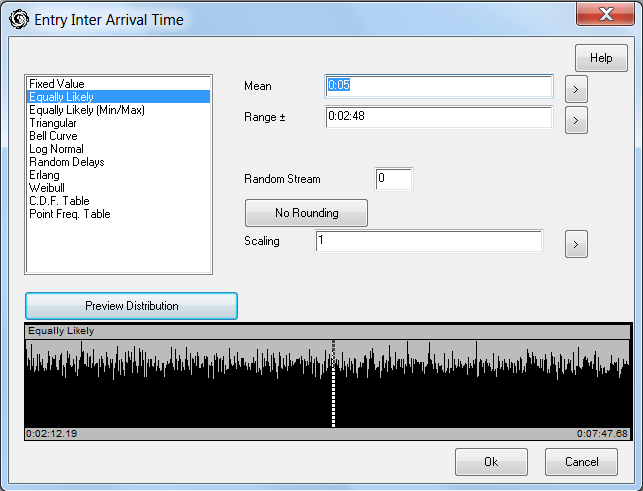
Inter-Arrival	5min 0sec	Equally Likely (aka Uniform Distribution)	2min 48sec
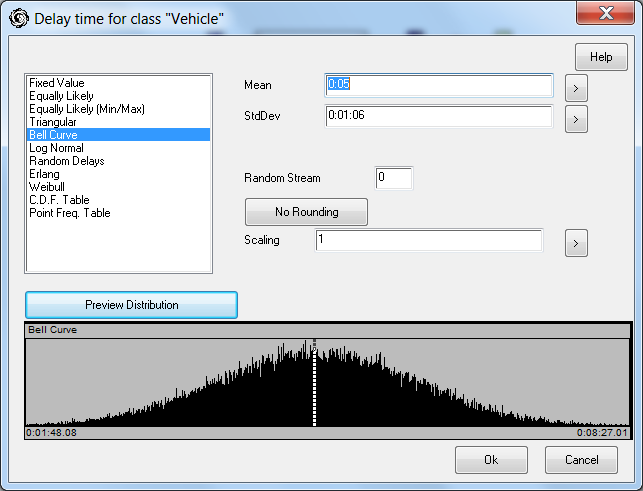
Load or Unload	5min 0sec	Bell Curve (aka Normal Distribution)	1min 6sec

Regardless of the variation pattern, we will keep the averages the same.

More Hands On

Go to Menu Bar / Edit / Interactions (Ctrl-I is a shortcut).

Notice the following things:

• The mouse pointer changes to show:
• (Interact) indicator in Planimate®’s Window Title.
• The Item Path appears in RED.

Click on the ENTRY

• Click the Pattern button next to Interval
• Configure the Distribution Pattern Dialog as above

(Equally Likely / Mean 0:5 / Range 0:2.48).

• Click on the Preview Plot button to View the distribution pattern.

• Click OK to close both dialogs.

Right click on the Load or Unload Server Object

• Select Bell Curve / Mean 0:5 / StdDev 0:1 06 in the Distribution Pattern Dialog.
• Click Preview Plot to View distribution pattern.

Notice the range of possible values in the sample plot. While the graph may show numbers less then zero the minimum will be clamped to 0 as time cannot go backwards.

Save, Run and Observe the Model

• Notice any new behaviour.
• Queuing now happens.
• Let us trace the queuing activity.

Go back to object mode (Ctrl-O) and right click on the Queue.

Select “Log Attributes To File”.

Tick the Queue 1 Occupancy row and OK the dialog.

Save and Run the model. Now click and pause the model (or press ESC).

We will now make use of the time acceleration features of Planimate®.

With the model paused, right click on the background of the model. The Advance to Time & Advance for Interval options enable you to ‘fast-forward’ the model up to a future point of time.

Select Advance For Interval in the background menu and enter “20d” in the dialog. This will advance for 20 days. After the advance (it will be quick) select “Pause”.

Viewing Results Graphically

Planimate models often contain graphs and views of data, but for simplicity in this tutorial we will use a pre-made Planimate application to study our model's performance.

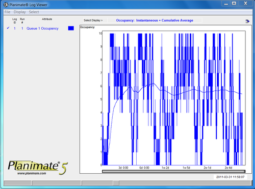
The “Log Attributes To File” option we selected earlier has caused the Queue's occupancy to be written to a log file.

Select menubar / Tools / Log Viewer. This will open another window, the Planimate Log Viewer application.

From its menu bar select File / Load Data. Browse to the folder where you saved the DC model, In this folder you should find dc01_01. Upon opening this file you will receive a “Log Data Successfully Loaded” message. OK It.

The viewer will switch to a new page and you will see Queue 1 Occupancy on the left. Click the cross in the left hand column, it will change to a tick and a graph will appear.

Notice the peak of the instantaneous graph is at 10. Lets examine this closer. Alt-tab back to Planimate and run model again. Use the Advance To Time again but this time select “Continue” instead of pause. Look closely at the Queue and Entry.

The default Queue has a capacity of 10 items, 5 visible and 5 indicated by the counter. You can see that the queue is full. This means the next item out of the Entry has nowhere to go and the Entry indicates this “blocked” situation by becoming red.

Blocking an Entry is bad for a simulation because it means items that were scheduled to arrive are not making it into the simulation.

RULE: Never Block an Entry because it will distort demand on your system.

Let’s try “fix” the system by adding a bigger queue capacity.